Neural Networks 2: Evaluation

In last week’s post, I introduced the Artificial Neural Network (ANN) algorithm by explaining how a single neuron in a neural network behaves. Essentially, we can think of a neuron as a classification algorithm with a number of inputs that correspond to the coordinates of data points and a single output that corresponds to the neuron’s prediction of the probability that the data point is in class 1, vs. class 0. I had originally planned to write a single second post about how things work when you connect neurons together, but after I started writing it, I decided to write separate posts about the training and evaluation phases of larger networks. As I explained last time, we need to understand the evaluation phase of a neural network before we can understand the training phase, so this week I’ll cover evaluation.

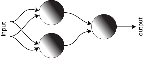
The rough idea that I alluded to last time was that we will form a neural network by connecting the outputs of some neurons to the inputs of others. An example of this is shown in the Figure below. To keep things simple, we will have each neuron use a logistic model/distribution on a two-dimensional data space, and we’ll assume that the parameters for each distribution are chosen at random. Once we’ve chosen the models, we classify a new data point as follows: We first feed the coordinates of the new data point into each of the two neurons on the left. Each neuron uses its stored logistic distribution to assign a value between 0 and 1 to that data point. These two values are then fed to the neuron on the right, which interprets them as coordinates in some other two-dimensional space. This neuron outputs the value of its own stored distribution for that new point and this value is the output of the whole network.

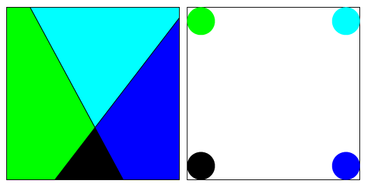
We would like to understand what’s going on from the geometric perspective, but in order to make things easier to see (and to draw), we will temporarily replace the logistic distribution in each of the two neurons with a distribution that is equal to exactly 1 on one side of a line (the decision boundary) and exactly zero on the other side. (This is sometimes called a step function.) The first two Neurons take their input directly from the original input, so they both define distributions on the “same” two dimensional data space. On the left in the Figure below, I’ve drawn the two distributions superimposed on each other, one in green and one in blue. The region where they are both zero is colored black. The region where only one of them is 1 is colored green or blue, respectively, and the region where they’re both equal to 1 is colored aqua blue (which is what you get when you combine green and blue in the RGB color scheme.)

The neuron on the right also keeps track of a distribution on a two-dimensional space, but this space is different from the data space that the first two neurons are interested in. As described above, the coordinates in the data space record the outputs of the first two neurons, so if you feed a given data point into the neural network, the coordinates that the neuron on the right sees describe which of the colored regions the data point lives in. The way that the colored regions correspond to coordinates is shown on the right side of the Figure. So, for example, if a data point is anywhere in the green region then the third neuron will see it as being in the upper left corner.

This is somewhat reminiscent of the way we used kernels: In order to create more complicated decision boundaries from linear classifiers, we transformed the initial data into a new coordinate system. The difference here is that the transformation defined by a neural network is not necessarily into a higher dimensional vector space. In fact, it’s much more common to actually decrease the dimension of the data space with neural networks.

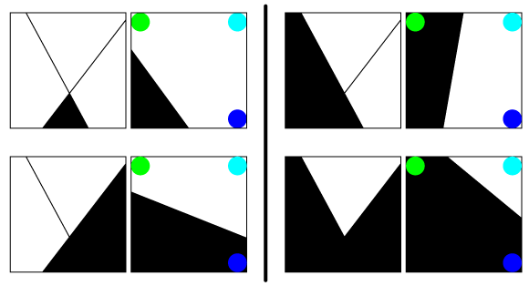
To see how this can give us a more complicated decision boundary, lets look at the possible decision boundaries for the third neuron and what they do to the distribution defined by the entire network. Some examples are shown below. In each case, the model used by the final neuron (shown on the right of each example) determines which of the four points will trigger an output of 0 or 1. From the above interpretation, we see that it’s really selecting which of the regions defined by the first two neurons get those labels (shown on the left of each example). The top right and bottom left examples are not particularly interesting: they’re just the linear models defined by the first two neurons. The interesting ones are the top left and bottom right, both of which are not linear.

So, somewhat like a kernel, the neural network allows us to define more complicated distributions than just ones with lines/planes/hyperplanes as their decision boundaries. However, while a kernel turns a single linear distribution into a more complicated shape, a neural network combines a number of simple models/distributions, in this case the linear models defined by the first two neurons.

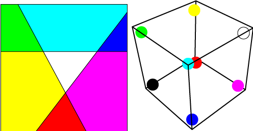
Note that the pictures really only show approximations of the final distributions that the network can determine, since we have a logistic distribution from each neuron, rather than a step distribution. The actual distribution has a smooth transition, which is roughly the result of blurring one of the distributions shown here. If we have more coordinates in our initial input and/or more neurons in the first layer (i.e. the neurons that get input directly from the data rather than from other neurons) then this will correspond to having higher dimensional distributions, with planes or hyperplanes as the decision boundaries. These will cut the initial higher dimensional data space into a number of regions, and the final neuron will select which regions correspond to 1s and which correspond to 0s. For example, if we have three neurons in our initial layer then the final neuron will have three dimensions of input and will have a collection of regions to choose from like the ones shown in the Figure below. The corresponding points in the three-dimensional vector space that the final neuron sees are shown on the right.

However, as long as we only have one layer of neurons, the final neuron will still be very limited in how it combines the regions that they define. The real power of neural networks comes from adding more layers in order to get more complicated patterns. For example, in the network drawn below (in which everything is two-dimensional), each of the neurons in the second layer can pick one of the distributions that the final neuron in the original network was allowed to (the ones shown in the third Figure). Then the very last neuron combines these second layer distributions to determine the network’s final answer. For example, you should see if you can work out how to choose distributions on the final three neurons that will pick out the blue and green regions (but not the black and aqua regions). Note that, as in the network below, while each neuron has a single output, this output can feed into the inputs of more than one other neuron.

So from this discussion, we start to see how to create interesting distributions by having layers of neurons, with each successive layer feeding into later layers. However, we’re also allowed to have more complicated networks, where connections can skip between layers, or there may not even be a well defined sense of layers at all. A few people have even developed schemes for having loops of neurons which feed back into each other, though this gets complicated and usually isn’t necessary. In any type of network, the connections between neurons determine what kinds of final distributions the neural network is capable of creating. The more neurons we have, the more complicated the distribution is allowed to be, and (repeating a common theme on this blog) the greater the risk of over-fitting. Larger networks are also more computationally expensive, though this seem to be less of an issue with modern computers. Designing a neural network that is both complicated enough to correctly model the data, but simple enough to avoid over-fitting is a combination of art and science.

But, of course, the real work of the neural network, namely finding a distribution that fits a given data set, is not done by designing the connections between the nodes: It’s done in the training phase, where each neuron in the network “learns” its distribution. I described a rough framework for this in the last post, but a more detailed discussion will have to wait for next week.