LSTMs

In past posts, I’ve described how Recurrent Neural Networks (RNNs) can be used to learn patterns in sequences of inputs, and how the idea of unrolling can be used to train them. It turns out that there are some significant limitations to the types of patterns that a typical RNN can learn, due to the way their weight matrices are used. As a result, there has been a lot of interest in a variant of RNNs called Long Short-Term Memory networks (LSTMs). As I’ll describe below, LSTMs have more control than typical RNNs over what they remember, which allows them to learn much more complex patterns.

Lets start with what I mean  by a “typical” RNN. In my post on RNNs, I mentioned three basic types of operations in the computation graph: 1) Outputs from nodes (which may be earlier or later in the network) can be concatenated into higher-dimensional vectors, for example to mix the current input vector with a vector that was calculated in a previous step. 2) Vectors can be multiplied by weight matrices, to combine and transform the concatenated vectors. 3) A fixed non-linear transformation can be applied to the output from each node in the computation graph.

The limitation with the RNNs defined by these three operations stems from the fact that while the weight matrices are updated during the training phase, they’re fixed while each sequence of inputs is processed. So each step in the input sequence is combined with the information stored from earlier steps in the same way each time. In some sense, the network is forced to remember the same things about each step in every sequence, even though some steps may be more important, or contain different types of information, than others.

An LSTM, on the other hand, is designed to be able to control what it remembers about each input, and to learn how to decide what to remember in the training phase. The key additional operation that goes into an LSTM is 4) Output vectors from nodes in the computation graph can by multiplied component-wise. In other words, the values in the first dimension of each vector are multiplied together to get the first dimension of a new vector. Then the second dimensions of the two vectors are multiplied, and so on.

This is not a linear transformation, in the sense that you can’t get the same result by concatenating the two vectors, then multiplying by a weight matrix. Instead, this is more like treating one of the input vectors as a  weight matrix that you’ll multiply the other output vector by. But unlike the weight matrices in a typical RNN, this “weight matrix” vector is determined by a computation somewhere else in the network, so it’s determined when the new data is processed, rather than fixed throughout the evaluation phase.

This “weight matrix” vector is in many ways not as impressive as one of the built-in weight matrices in a typical RNN. It’s equivalent to a matrix with the values of the vector along the diagonals, and the rest of the entries equal to zero. So it can’t do anything fancy to the other vector. Instead, you should think of it as a sort of filter that decides what parts of the other vector are important. In particular, if the “weight matrix” vector is zero in a given dimension then the result of multiplication will be zero in that dimension, no matter what the value was for that dimension in the other vector. If it’s close to 1, the output value is exactly equal to the value of the other vector in that dimension. (And a non-linear transformation is often applied to make sure the “weight matrix” values are very close to either 0 or 1.) So the “weight matrix” vector chooses what parts of a second vector get passed on to the next step. Because of this, the nodes in the computation graph where a “weight matrix” vector gets multiplied by a data vector is often called a gate.

An LSTM uses this fancy new fourth operation to create three gates, illustrated in the Figure below. This shows the inside of a single cell in an LSTM, and we’ll see farther down how this cell gets hooked up on the outside.

The LSTM cell has two inputs and two outputs. The output at the top (labeled out) is the actual RNN output, i.e. the output vector that you will use to evaluate and train the network. The output on the right (labeled mem) is the “memory” output, a vector that the LSTM wants to record for the next step. Similarly, the input on the bottom (labeled in) is the same as the input to a standard RNN, i.e. the next input vector in the sequence. The input on the right (also labeled mem) is the “memory” vector that was output from the LSTM cell during the previous step in the sequence. You should think of the LSTM as using the new input to update the value of the memory vector before passing it on to the next step, then using the new memory value to generate the actual output for the step.

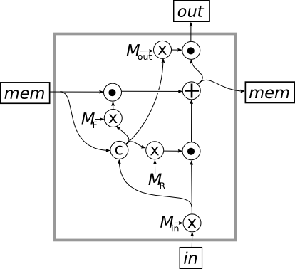When a new input vector comes in through the bottom of the LSTM, it is multiplied by the weight matrix , which puts it into the same form as the memory vector. We want to combine this with the memory vector using gates like we described above. So the input vector is also concatenated with the previous cycle’s memory vector, and this is multiplied by three different weight matrices: controls what the cell “remembers” about the input, controls what the cell “forgets” from memory and controls what part of the current memory is output at the top. The results of each multiplication are fed through a non-linear transformation that I didn’t include in the Figure.

Then these vectors are fed into gates, defined by our new network operation (indicated by a circle with a dot in it) as shown in the Figure. The middle gate filters the memory vector from the previous step and the bottom gate filters the transformed input vector. These two gated vectors are then added together to produce the memory vector for this step. In addition to becoming the memory vector that is sent to the next step in the LSTM, the memory vector is also filtered by the top gate to produce the actual output from the LSTM.

The key step in this process is how the memory vector and the transformed input vector are independently gated before being added together. In the simplest setup, each of the “weight matrix” vectors would have all their values 0 or 1, and these would be complementary between the two gates, so that each dimension gets the value from one or the other. The values, which are calculated from both the current input and the current memory vector, would thus determine which of the dimensions in the memory vector should be passed on to the next step, and which should be replaced with the corresponding value from the transformed input vector. But in practice, the network gets to “learn” whatever behavior is most effective for producing the desired output patterns, so it may be much more complex.

Speaking of which, lets quickly look at how an LSTM is trained, using the idea of unrolling that I described in my previous post. As you probably picked up from the discussion above, we hook up an LSTM externally by adding an edge from the right memory out, back around to the left memory in. This is shown on the left in the Figure below. This edge is a bit unwieldy to draw, wrapping around behind the cell. But once you unroll the network, as on the right of the Figure, it forms a nice, neat, horizontal edge from each step in the LSTM to the next.

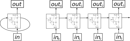
As with a standard RNN, you can use unrolling to understand the training process, by feeding the whole sequence of inputs to the network at once, and using back propagation to update the weight matrices based on the desired sequence of outputs.

Note that LSTMs are fairly “shallow” as neural networks go, i.e. there aren’t that many layers of neurons. In fact, if you ignore the gates, there is a single lonely weight matrix between the input vector and the output vector. Of course, there are a number of ways one could modify an LSTM to make it more flexible, and a number of people have experimented with “deep LSTMs”. But for now, I’ll leave that for the readers’ imaginations, or maybe a future post.