Rolling and Unrolling RNNs

A while back, I discussed Recurrent Neural Networks (RNNs), a type of artificial neural network in which some of the connections between neurons point “backwards”. When a sequence of inputs is fed into such a network, the backward arrows feed information about earlier input values back into the system at later steps. One thing that I didn’t describe in that post was how to train such a network. So in this post, I want to present one way of thinking about training an RNN, called unrolling.

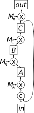
Recall that a neural network is defined by a directed graph, i.e. a graph in which each edge has an arrow pointing from one endpoint to the other. In my earlier post on RNNs, I described this graph in terms of the classical neural network picture in which each vertex is a neuron that emits a single value. But for this post, it’ll be easier to describe things in the tensor setting, where each vertex represents a vector defined by a row/layer of neurons. That way, we can think of our network as starting with a single vertex representing the input vector and ending at a single output vertex representing the output vector. We can get to every vertex in the graph by starting from this input vertex and following edges in the direction that their arrows point. Similarly, we can get from any vertex to the output vertex by following some path of edges.

A standard (non-recurrent) feed-forward network is a directed acyclic graph (DAG) which means that in addition to being directed, it has the property that if you start at any vertex and follow edges in the directions that the arrows point, you’ll never get back to where you started (acyclic). As a result there’s a natural flow through the network that allows us to calculate the vectors represented by each vertex one at a time so that by the time we calculate each vector, we’ve already calculated its inputs, i.e. vectors on the other ends of the edges that point to it.

In an RNN, the graph has cycles, so no matter how we arrange the vertices, there will always be edges pointing backwards, from vertices whose vectors we haven’t yet calculated. But we can deal with this by using the output from the previous step.

For example, the vector  in the Figure to the right is calculated from the input vector and the intermediate vector  (multiplied by a weight matrix ). The circle with the ‘c’ in it represents concatenating the vectors  and , which means creating a new (higher dimensional) vector where the first half of the entries come from the input vector and the second half come from .

When the first input value gets to vertex , we don’t yet have a value to use for , so we’ll just use the zero vector of the appropriate dimension, and we’ll let be the value that we calculate. Similarly, we can calculate by multiplying  by the matrix and the first output value from and .

Then comes the second value in the input sequence, which we’ll call . When we go to calculate , we haven’t yet calculated , but we do have lying around from the last step. So we’ll calculate using and . Then we can calculate and . This will be used to calculate in the next step, and so on.

In order to better understand what’s going on here, lets draw a new graph that represents all the values that we’ll calculate for the vertices in the original graph. So, in particular  and will be two separate vertices in this new graph, and an edge goes from to the concatenation operator that leads into vertex . This is shown in the Figure below for the first four steps in an input sequence.

 

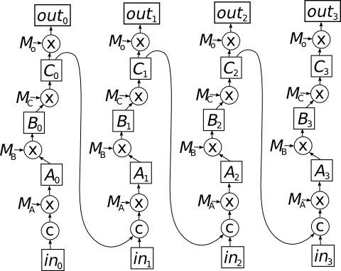
The first thing you should notice about this graph is that it has multiple inputs – one for each vector in the input sequence – and multiple outputs. The second thing you might have noticed is that this graph is acyclic. In particular, the cycle that characterized the original graph has been “unrolled” into a longer path that you can follow to the right in the new graph.

(For any readers who have studied topology, this is nicely reminiscent of the construction of a universal cover. In fact, if you unroll infinitely in both the positive and negative directions, the unrolled graph will be a covering space of original graph. And as noted above, it will be acyclic (in terms of directed cycles, though not necessarily undirected cycles), which is analogous to being simply connected. So maybe there’s some category theoretic sense in which it really is a universal cover… but I digress.)

It turns out you can always form a DAG from a cyclic directed graph by this procedure, which is called unrolling. Note that in the unrolled graph, we have lots of copies of the weight matrices . These are the same at every step in the sequence so they don’t get unrolled.

However, we do need to update the weight matrices in order to train the neural network, and this is where the idea of unrolling really comes in handy. Because the unrolled network is a DAG, we can train it using back-propagation just like a standard neural network. But the input to this unrolled network isn’t a single vector from the sequence – it’s the entire sequence, all at once! And the target output we use to calculate the gradients is the entire sequence of output values we would like the network to produce for each step in the input sequence. In practice, it’s common to truncate the network and only use a portion of the sequence for each training step.

In the back-propagation step, we calculate gradients and use them to update the weight matrices . Since we have multiple copies of each weight matrix, we’re probably going to get different gradients for each copy. But we want all the copies of each matrix to stay the same, so we’ll combine all the gradients, usually by taking an average, and use this to update the base matrix that all the copies are taken from.

In practice, you don’t necessarily need to explicitly construct the unrolled network in order to train an RNN with back-propagation. As long as you’re willing to deal with some complex book keeping, you can calculate the gradients for the weight matrices directly from the original graph. But nonetheless, unrolling is a nice way to think about the training process, independent of how it’s actually done.