Principal Component Analysis

Now that we’ve gotten a taste of the curse of dimensionality, lets look at another potential problem with the basic form of regression we discussed a few posts back. Notice that linear/least squares regression always gives you an answer, whether or not that answer is any good. If you want to find a line that best fits your data, the regression algorithm will give you a line, regardless of the actual structure of the data. So what we also need is a way to determine how good the model discovered by regression is at approximating the data. There are a few different ways to do this, and in this post, I’ll introduce one called Principal Component Analysis (PCA).

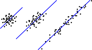
One of the main goals of PCA is to tell the difference between the three data sets shown to the left. If you run linear regression on each of them, you’ll get the same line, shown in blue. But there’s clearly a difference in how well this line approximates each data set – It does a really good job of summarizing the data set on the right, but a pretty miserable job for the data set on the left. For the middle data set, it’s somewhere in between. We can see the difference for a two-dimensional data set, but as usual we won’t be able to visually inspect the data like this if there are more dimensions. That’s where PCA comes in.

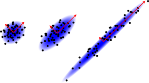
PCA can tell the difference between these three sets because rather than fitting a line or a plane or a hyperplane to the data, it (roughly speaking) fits an elliptical Gaussian distribution, such as those shown in the second picture. This distribution is defined by its axes or principal components – the red arrows shown in each picture. The angles of these vectors tell you the angle that the cloud is tilted at and the lengths of the vectors tell you how much it is stretched in each direction. The arrows on the left are almost the same length, but on the right, one of the arrows is much longer than the other. This large difference in length is what tells us that the data set on the right is much closer to a line along the longer vector.

This is probably a fitting place to remind the reader of one common misconception: PCA and any other computational/statistical method only measures correlations in the data, not causation. So no matter how closely the data fits a given model, I would be wrong to conclude that one factor or set of factors causes another. If two things are correlated, it might that one causes the other or it might mean that both are caused by an external factor not represented in the data. But a correlation could also be a coincidence or the result of a bias in the way the data was collected. One can sometimes establish causation by running controlled experiments, but no amount data analysis alone can turn a correlation into a causation.

OK, now that that’s out of the way, lets consider higher dimensional PCA. Because the examples above are two-dimensional data sets, there are two axes and two vectors. For higher dimensional data sets, there will be more axes. In particular, for an n-dimensional data set there will be n principal components. Some of these will be very short and some will be long, and the interpretation of long and short will be the same as in the two-dimensional case. So even though we won’t be able to see a high dimensional data set the same way we see a two-dimensional data set, we can get a rough idea of its shape from the principal component vectors.

For example, if we have a fifteen-dimensional data set with three really long PCA vectors and twelve really short vectors, then that means the data is mostly concentrated along a  three-dimensional hyperplane in a fifteen-dimensional space. Moreover, those three long principal components define this three-dimensional hyperplane along which the data lies. As in the picture, each principal component usually won’t be along one of our original features (though occasionally they might.) Instead, they will define some interesting correlations between combinations of features. (But again, we should never conclude that the value of one feature determines the value of another just because they’re strongly correlated.)

Unlike the form of regression that we discussed previously, PCA does not work by formally fitting a model to the data. Instead, it works by calculating the principal components directly from the structure of the data. The PCA algorithm is usually described in terms of variances and covariances between the different features/dimensions that define the space that the data lives in. But I want to explain it from a different perspective that leads to the same algorithm, but is a more geometrically intuitive. It also involves ideas that will come up later on in this blog.

We start by centering the data in our n-dimensional space. In other words, we find the center of mass in each direction, then translate the entire data set so that the center of mass in each direction is at exactly zero.

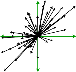
Next, we want to think of each data point as pulling on the data set, attempting to stretch it away from the origin, as indicated on the right. (The green arrows are the axes.) Note that the data points aren’t pulling away from each other – they’re pulling away from the center of mass. The farther a point is from the center of mass, the harder it pulls. With each point pulling together, we want to consider the overall effect that they have on the set. In particular, if there are a lot of points far away from the origin in one direction, as in the data set on the right of the above figures, the data set will mostly get pulled in that direction. Because it’s a stretching action rather than a translation, points that are pulling in opposite directions are actually working with each other rather than against each other.

The forces of all this pulling can be summarized in a certain matrix (which happens to be equal to the covariance matrix from statistics.) A direction in which the points are pulling the hardest is called that first eigenvector of the matrix and this will be the longest principal component. Next we look at all the vectors that are orthogonal/perpendicular to the first eigenvector and choose a direction with the most force among these, which we call the second eigenvector. The we look at all the vectors that are orthogonal/perpendicular to the first two eigenvectors and so on until we run out of orthogonal vectors.

The length of each eigenvector will indicate how strongly the data is pulling things in that direction. In practice, these vectors are calculated by a process called diagonalizing the initial matrix. So the PCA algorithm consists of calculating this matrix, diagonalizing it, then translating the results into principal component vectors.

The PCA gives you a lot more information than linear regression, but note that it does not have the flexibility of the types of regression we discussed with curved hyperplanes. So if your data follows a curved shape rather than a hyperplane, PCA may give you lousy results. There are ways to fix this, such as something called a kernel, but that will have to wait for a later post.